
Installing BFEE2 can be done with Conda using the following line
conda install -c conda-forge BFEE2Preparing Systems for Input to BFEE2
To take the flooding systems and prepare them for BFEE2 there are a few post-processing steps that need to be completed. While flooding saves PDB files without the waters and ions, we want to retain these from the simulations in order to capture any trapped waters or other important features from the system. To do this you will need to find the frame of the trajectory using the .site file made during flooding. This ends with a best line that shows the trajectory, frame number, and ligand number that was used to make the site
BEST: ../../beta_arrestin_2_flooding/dcme_neutral_flooding/arrestin2_dcme_neutral_4.dcd 1628 43From there you will want to use frame2pdb from LOOS to make the new PDB file with all the waters. Below is the usage for frame2pdb where the model will be the prmtop used to run the systems
Usage- frame2pdb [options] model trajectory frameno So from that a specific line to make the new pdb file may look like what is shown below. You will need to direct the output to a file otherwise it will just output the pdb onto your screen
frame2pdb arrestin_dcme_neutral_hmr.prmtop arrestin2_dcme_neutral_4.dcd 1628 > frame.pdbFrom here there remain two problems:
1. This still contains all the ligands used for flooding, not just the 1 ligand bound
2. BFEE2 does not work with a 4 point water model (like OPC) used here and the waters need to be converted to the 3 point model OPC3
Below is a link to download a code called extract_convert.py that solves both of these problems. It will also re-neutralize the system for any charged ligand systems so that there isn’t a net charge after the ligands have been removed
Usage of this code would look something like the following:
extract_convert.py usage: python extract_convert.py input_structure ligand_name ligand_number ligand_charge output_structure

--(input/output)_structure arg ---PDB

--ligand_name arg ---string ligand name in input file

--ligand_number arg ---int (representing residue number in input file)

--ligand_charge arg ---int (-1,0,1)
There is one change that the code does not make for you, you need to add “TER” after the final line with the ligand otherwise it will cause errors in tleap
Now that you have a correct PDB file for your system you have to make a prmtop and rst7 file for this system, and also add HMR into the prmtop file. To make the original prmtop and rst7 you will run the PDB through tleap using the following linked input file. You will just have to change the input lines for your PDB file and what your desired output file names would be. The complex box should be set to match whatever box size was used in the flooding simulations. The .lib and .frcmod files are from the ligand for flooding simulations and you should still have these available from flooding setup.
Usage: tleap -f tleap.in
Finally to add HMR you will take the prmtop and rst7 from tleap and run them through parmed in amber. You will input the two files as shown below
parmed -p bfee2_input.prmtop -c bfee2_input.rst7Once ParmEd opens you will run the following lines:
>HMassRepartition
Repartitioning hydrogen masses to 3.024 daltons. Not changing water hydrogen masses.
>parmout bfee2_input_hmr.prmtop bfee2_input_hmr.rst7
>go
Creating and Running BFEE2 Simulation Files
Now that you have a prmtop and rst7 file ready to input to BFEE2 you can generate the simulation files and system files for running BFEE2. BFEE2 generates all inputs using a GUI which can be opened by running the following line in terminal with your bfee2 Conda environment activated:
BFEE2Gui.pyThat will then open a window that looks like this:

This pre-treatment tab is what will be used to generate the simulation files. You will need to browse for the input prmtop and rst7, change the forcefield type to Amber, set the selection strings for the protein and the ligand, and then finally change the strategy to Alchemical. An example is shown below:
NOTE: The given selection string will not work for beta Arrestin systems after they have gone through extract_convert.py. Where that script puts the ligand first you want your protein selection string to be resid 2-389 for beta Arrestin 1 or 2-401 for beta Arrestin 2. For non-arrestin systems your selection string would be 2-end of protein

After hitting generate inputs if all goes successfully you will then see the pop-up window shown above. This then creates a new folder called BFEE. You will want to rename this folder as it will be overwritten each time you run BFEE2, and you will need to keep track of which folders have which systems in them. The folder generated will look something like what is shown below:
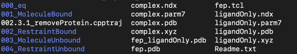
IMPORTANT NOTE: DO NOT CHANGE ANY OF THE FILE NAMES IN THE FOLDER. The BFEE2 code looks specifically for the file names that it generates. There may be a few small examples where file names need to be changed that will be discussed later, but you will also have to change conf files and other things to do so. For the most part keep all file names the same.
Readme.txt contains steps for the order to run the simulations, as well as one extra step for amber users that will be important to do in order to run any of the ligand only simulation steps
Here are the contents of Readme.txt:
To calculate the binding free energy:
1.1. run 000_eq/000.1_eq.conf
1.2. (optionally) run 000_eq/000.3_updateCenters.py
2.1. run 001_MoleculeBound/001.1_fep_backward.conf
2.2. run 001_MoleculeBound/001.2_fep_forward.conf
3.1. run 002_RestraintBound/002.1_ti_backward.conf
3.2. run 002_RestraintBound/002.2_ti_forward.conf
4.1. CHARMM user:
(if you didn’t link BFEE with VMD before generating inputs)
run 002.3_removeProtein.tcl using VMD
Amber user:
run 002.3_removeProtein.cpptraj using cpptraj
4.2 run 000_eq/000.2_eq_ligandOnly.conf
4.3. run 003_MoleculeUnbound/003.1_fep_backward.conf
4.4. run 003_MoleculeUnbound/003.2_fep_forward.conf
5.1. run 004_RestraintUnbound/004.1_ti_backward.conf
5.2. run 004_RestraintUnbound/004.2_ti_forward.conf
(steps 2-5 can be done in parallel)
6. do post-treatment using BFEE
It is correct that steps 2-5 can be run in parallel, but you must make sure that the backward simulation is complete before the corresponding forward simulation. The end point of the backward simulation is the starting point of the forward simulation and the forward simulation will not run if its corresponding backward simulation is not complete. I also recommend running what they call step 4.1 first so that way both sets of equilibration steps can be done and then all simulations from the 001,002,003, and 004 folders can be run simultaneously but you can run these following the steps outlined above as well.
For using cpptraj you need to make sure you have an amber module loaded and then run:
cpptraj 002.3_removeProtein.cpptrajHow to actually run these simulations will be covered in the running on bluehive section, but before any simulations can be run there are edits needed to the namd input files from what was generated by BFEE2
Editing The “.conf” Files
Each folder will have a .conf file – these are the input files for NAMD. There are a few changes that will need to be made to make sure these systems will run correctly. The beginning of the .conf file should look as follows, if any of the lines are not there make sure to add them to each file. The parmFile – bondedCuda lines are the Amber specific lines that may be missing but the rest is added for context to know where to look in the file
coordinates    ../complex.pdb
parmFile      ../complex.parm7
amber    on
usePMECUDA on
CUDASOAintegrate on
alchPMECUDA on
bondedCUDA 255
exclude    scaled1-4
1-4scaling    0.83333333
switching            on
Additionally you will have to specify that a 3 point water model is being used by adding a water model line in the section with other water parameters, which will look like this after edits:
wrapAll              off
wrapWater            on
waterModel           tip3
langevin             on
Even though we are using OPC3 just list tip3 as it only cares to specify if it is a 3point or 4point water model. The actual parameters are included in the .parm7 file that it loads in at the beginning
You also will need to update the tilmestep line to be 4fs for the HMR timestep. The default value is 2fs, after edits the line should look as follows
PMETolerance         10e-6
PMEInterpOrder       4
PMEGridSpacing       1.0
timestep             4.0
fullelectfrequency   2
nonbondedfreq        1
These specific changes must be made to ALL CONF FILES IN ALL FOLDERS
Due to runtime limits and longer runs for the 001 folder simulations these conf files need to be split into two separate simulations. For these simulations you run half the lambda windows as one simulation and half as another simulation. In doing so these folders will have 4 separate conf files, like what is shown below:

Formatting for each will be very similar – here is an example of one of the backward conf files so you can also see other previously mentioned changes included. You need to make sure to update each output name to be unique and in the runFEP line change the lambda range for the half of the simulation this file corresponds too, as well as double the runtime from 500000 to 10000000.
coordinates    ../complex.pdb
parmFile      ../complex.parm7
amber    on
usePMECUDA on
CUDASOAintegrate on
alchPMECUDA on
bondedCUDA 255
exclude    scaled1-4
1-4scaling    0.83333333
switching            on
switchdist           8.0
cutoff               9.0
pairlistdist         11.0
bincoordinates    ../000_eq/output/eq.coor
binvelocities    ../000_eq/output/eq.vel
ExtendedSystem    ../000_eq/output/eq.xsc
binaryoutput         yes
binaryrestart        yes
outputname           output/fep_backward_0.5-0.0
dcdUnitCell          yes
outputenergies       5000
outputtiming         5000
outputpressure       5000
restartfreq          5000
XSTFreq              5000
dcdFreq              5000
hgroupcutoff         2.8
wrapAll              off
wrapWater            on
waterModel           tip3
langevin             on
langevinDamping      1
langevinTemp         300.0
langevinHydrogen     no
langevinpiston       on
langevinpistontarget 1.01325
langevinpistonperiod 200
langevinpistondecay  100
langevinpistontemp   300.0
usegrouppressure     yes
PME                  yes
PMETolerance         10e-6
PMEInterpOrder       4
PMEGridSpacing       1.0
timestep             4.0
fullelectfrequency   2
nonbondedfreq        1
rigidbonds           all
rigidtolerance       0.00001
rigiditerations      400
stepspercycle        10
splitpatch           hydrogen
margin               2
useflexiblecell      no
useConstantRatio     no
colvars    on
colvarsConfig    colvars.in
source ../fep.tcl
alch on
alchType FEP
alchFile ../fep.pdb
alchCol B
alchOutFile output/fep_backward_0.5-0.0.fepout
alchOutFreq 50
alchVdwLambdaEnd 0.7
alchElecLambdaStart 0.5
alchEquilSteps 100000
runFEP 0.5 0.0 -0.02 1000000
Next here is an example of the corresponding forward simulation to that lambda range. There are more changes to make for the forward simulations as you must make sure they reference the correct set of backwards simulations.
coordinates    ../complex.pdb
parmFile      ../complex.parm7
amber    on
usePMECUDA on
CUDASOAintegrate on
alchPMECUDA on
bondedCUDA 255
exclude    scaled1-4
1-4scaling    0.83333333
switching            on
switchdist           8.0
cutoff               9.0
pairlistdist         11.0
bincoordinates    output/fep_backward_0.5-0.0.coor
binvelocities    output/fep_backward_0.5-0.0.vel
ExtendedSystem    output/fep_backward_0.5-0.0.xsc
binaryoutput         yes
binaryrestart        yes
outputname           output/fep_forward_0.0-0.5
dcdUnitCell          yes
outputenergies       5000
outputtiming         5000
outputpressure       5000
restartfreq          5000
XSTFreq              5000
dcdFreq              5000
hgroupcutoff         2.8
wrapAll              off
wrapWater            on
waterModel           tip3
langevin             on
langevinDamping      1
langevinTemp         300.0
langevinHydrogen     no
langevinpiston       on
langevinpistontarget 1.01325
langevinpistonperiod 200
langevinpistondecay  100
langevinpistontemp   300.0
usegrouppressure     yes
PME                  yes
PMETolerance         10e-6
PMEInterpOrder       4
PMEGridSpacing       1.0
timestep             4.0
fullelectfrequency   2
nonbondedfreq        1
rigidbonds           all
rigidtolerance       0.00001
rigiditerations      400
stepspercycle        10
splitpatch           hydrogen
margin               2
useflexiblecell      no
useConstantRatio     no
colvars    on
colvarsConfig    colvars.in
source ../fep.tcl
alch on
alchType FEP
alchFile ../fep.pdb
alchCol B
alchOutFile output/fep_forward_0.0-0.5.fepout
alchOutFreq 50
alchVdwLambdaEnd 0.7
alchElecLambdaStart 0.5
alchEquilSteps 100000
runFEP 0.0 0.5 0.02 1000000
Again here the lambda range and runtime have been updated but the velocities and coordinates used at the start are from the previous backward simulation so you have to reference that correctly. For the lambda range 0.5-1.0 you will just switch the values around so the conf files reference that range instead
Once the .conf file edits have been made you can then submit the simulations on bluehive.
Running the Simulations on Bluehive
Here is an example script that runs both equilibrations. You will have needed to run the cpptraj line for the ligand simulations first before running this script.
#!/bin/bash
#SBATCH -p gpu -C A100|V100 --gres=gpu:1  -t 5-00:00:00 -c 1 --mem=4gb -J Equilibrate -o equil.out
#module load namd/3.0b3
module load gcc/9.1.0 cuda/11.3
export CUDA_BIN_PATH=/software/cuda/11.3/usr/local/cuda-11.3/bin/nvcc
export CC=/software/gcc/9.1.0/b1/bin/gcc
export CXX=/software/gcc/9.1.0/b1/bin/g++

/scratch/agrossfi_lab/software/namd3-b6/namd3 +p1 +idlepoll +devices $CUDA_VISIBLE_DEVICES 000.1_eq.conf > 000.1_eq.log
/scratch/agrossfi_lab/software/namd3-b6/namd3 +p1 +idlepoll +devices $CUDA_VISIBLE_DEVICES 000.2_eq_ligandOnly.conf > 000.2_eq_ligandOnly.log
I have also written some scripts to submit production jobs as well as pair the forward and backward simulation so that the forward simulation will run after the backward simulation finishes. Here is an example of one of these scripts:
#!/bin/bash
#SBATCH -p gpu -C A100|V100 --gres=gpu:1  -t 5-00:00:00 -c 1 --mem=4gb -J MB_BW -o MB_
backward.out
#module load namd/3.0b3
module load gcc/9.1.0 cuda/11.3
export CUDA_BIN_PATH=/software/cuda/11.3/usr/local/cuda-11.3/bin/nvcc
export CC=/software/gcc/9.1.0/b1/bin/gcc
export CXX=/software/gcc/9.1.0/b1/bin/g++

/scratch/agrossfi_lab/software/namd3-b6/namd3 +p1 +idlepoll +devices $CUDA_VISIBLE_DEVICES 001.1_fep_backward.conf > 001.1_fep_backward.log

mb_forward=/scratch/erobin20/bfee2_fe_calcs/barr1_dcma_charged_bfee2/bfee2_replica_2/001_MoleculeBound/mb_forward.sbatch

cat > $mb_forward <<EOF
#!/bin/bash
#SBATCH -p gpu -C A100|V100 --gres=gpu:1  -t 5-00:00:00 -c 1 --mem=4gb -J MB_FW -o MB_forward.out
module load gcc/9.1.0 cuda/11.3
export CUDA_BIN_PATH=/software/cuda/11.3/usr/local/cuda-11.3/bin/nvcc
export CC=/software/gcc/9.1.0/b1/bin/gcc
export CXX=/software/gcc/9.1.0/b1/bin/g++

/scratch/agrossfi_lab/software/namd3-b6/namd3 +p1 +idlepoll +devices $CUDA_VISIBLE_DEVICES 001.2_fep_forward.conf > 001.2_fep_forward.log
    /
EOF

chmod +x $mb_forward

sbatch $mb_forward
The lab has our own build of the namd3 beta that works best with BFEE2 and Colvars so it is important to have the full call line to namd3. The exports also make sure that we have the correct Cuda and compilers for using this version of namd so you will need to leave those in as well. Finally, this version of namd only works on the A100, V100, or Grossfield T4 GPUs so you need to make sure that they are selected correctly in the sbatch line otherwise there will be Cuda issues and your simulation will not run. You will need one of these scripts for each folder (001, 002, 003, and 004). These can only be run once the equilibration is complete so make sure you have already run that script and it completed successfully
Replicates of Simulations
For all of these systems it is important to run replicates for error estimates. The current replica scheme that we have found effective for sampling is as follows:
- 3 Replicas of Equilibration per system
- 3 Replicas of Simulations Run in the 003 and 004 folders
- 6 total Replicas of Simulations Run in the 001 and 002 Folders (2 started per corresponding equilibration)
You do not have to build 3 separate times in BFEE2 for the different equilibrations, just copy the original output folder from BFEE2 to have 3 total copies of the folder
Post Processing Simulations using BFEE2
BFEE2 doesn’t intend on having simulations split, so you have to first concatenate the outputs from the 001 window simulations into one backward output file and one forward output file. To do this you will run the two following lines:
cat fep_backward_1.0-0.5.fepout fep_backward_0.5-0.0.fepout > 001_fep_backward.fepout

cat fep_forward_0.0-0.5.fepout fep_forward_0.5-1.0.fepout > 001_fep_forward.fepout
You can name these files whatever you like but I prefer adding the 001 marker as the outputs from the 003 files are also called fep_backward.fepout and fep_forward.fepout respectively and it can get confusing or you risk overwriting files.
The BFEE2 Gui is used to complete the free energy calculation. You will again open up the gui but switch to the post-treatment tab and click on Alchemical
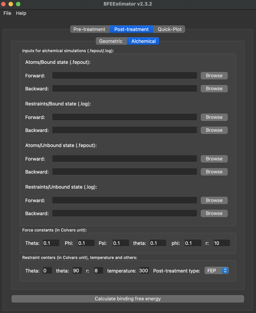
For the Atoms bound and unbound states you will be using an .fepout file which will be found in the output folder of the folder where you ran the simulation. An example of the 001_MoleculeBound folder and some of the output folder is shown below – this corresponds to the Atoms/Bound state for inputing files to BFEE2
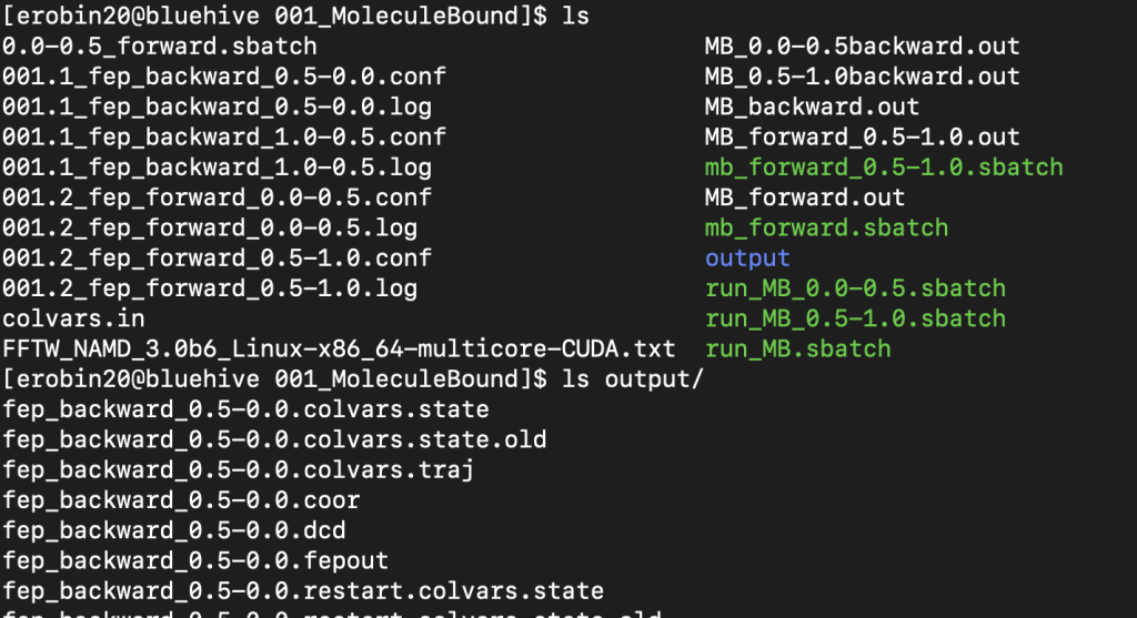
This output folder shows the files before concatenation but you will expect to see files like this before running that line. The concatenated file is the relevant one from the 001 folder and from 003 folders again you expect to see fep_backward.fepout and fep_forward.fepout as your relevant files
For the 002 and 004 folders those represent the restraints bound and unbound respectively. For those you will just use the .log file generated next to the .conf file in those folders, you will not need to add anything from the output folder. Once all files are uploaded into the GUI you just have to change the Post-Treatement Type and the bottom from FEP to BAR, and can then hit the calculate binding free energy button. If there are no errors in inputs you will then get a popup window with the free energy value calculated from the simulation, which will contain information printed out as follows:
Results:
ΔG(site,couple)   = 34.87 ± 0.06 kcal/mol
ΔG(site,c+o+a+r)  = -9.77 ± 0.52 kcal/mol
ΔG(bulk,decouple) = -41.13 ± 0.07 kcal/mol
ΔG(bulk,c)        = 3.94 ± 0.35 kcal/mol
ΔG(bulk,o+a+r)    = 11.51 kcal/mol
Standard Binding Free Energy:
ΔG(total)         = -0.59 ± 0.64 kcal/mol